Learning based models for Classification

Thousands of learning algorithms have been developed in the field of machine learning. Scientists typically select from among these algorithms to solve specific problems. Their options are frequently limited by their familiarity with these algorithms. In this classical/traditional machine learning framework, scientists are forced to make some assumptions in order to use an existing algorithm. While this can be limiting in some scenarios, it can offer the benifit of speed, low cost computing and ease of use as a tradeoff for overfitting and reduced accuracy.

In this article, we have built multiple learning based models for Classification on Sequential data (ECG) to detect the probability of heart disease. Ensemble Learning, Support Vector Machines, Bernoulli Nave Bayes, K Nearest Neighbor, and the Random Forest Classifier are explored in great depth for our classification task. You can check out the code and the dataset in this repository .

Naïve Bayes

The Naive Bayes classifier divides data into classes using Bayes’ Theorem and the assumption that all predictors are independent of one another. It is assumed that the presence of one feature in a class is unrelated to the presence of other features.

For example, if a fruit is green, round, and has a 10-inch diameter, it is a watermelon. These characteristics may be mutually exclusive, but each one independently contributes to the likelihood that the fruit under consideration is a watermelon. That is why the term ‘Naive’ appears in the name of this classifier.

Here is the Bayes theorem, which serves as the foundation for this algorithm:

P(c|x) = P(x|c) * P(c)/P(x)

In this equation, ‘c’ represents class and ‘x’ represents attributes. P(c/x) represents the predictor’s posterior probability of class. P(x) is the predictor’s prior probability, and P(c) is the class’s prior probability. P(x/c) represents the predictor’s probability based on the class.

How can it be used for our dataset?

We will be using a particular version of Naïve Bayes called the Bernoulli Naive Bayes. The predictors in this case are boolean variables. So our options are ‘True’ and ‘False’ (True for Heart Disease, or Not True for Heart Disease).

It is one of the most common types of Naive Bayes models: Its operation is identical to that of the Multinomial classifier. The predictor variables, on the other hand, are the independent Boolean variables. For example, it can determine whether a specific word exists or not in a document. BernoulliNB is designed for binary/boolean features. Since our Feature set is a discrete set of binary values, Bernoulli Naive Bayes is particularly suited for predicting heart disease from our dataset.

K-nearest neighbour

The k-nearest neighbours (KNN) algorithm is a data classification method that estimates the likelihood that a data point will belong to one of two groups based on which data points are closest to it.

The supervised machine learning algorithm k-nearest neighbour is used to solve classification and regression problems. However, it is primarily used to solve classification problems.

Consider the following two groups: A and B.

The algorithm examines the states of data points nearby to determine whether a data point belongs in group A or group B. If the majority of data points are in group A, the data point in question is almost certainly in group A, and vice versa.

In a nutshell, KNN entails classifying a data point by examining the nearest annotated data point, also known as the nearest neighbour.

How can it be used for our dataset?

When KNN is used for classification, the output is the class with the highest frequency among the K-most similar instances. In essence, each instance votes for their class, and the class with the most votes is selected as the prediction.

Class probabilities can be calculated as the normalised frequency of samples in the set of K most similar instances for a new data instance that belongs to each class. In a binary classification problem (class is either 0 or 1), for example,

p(class=0) = count(class=0) / count(class=0) + count(class=1)

We have used a range of values for K (np.arange(1, 25, 2)) and let the GridSearchCV find the best parameter for n_neighbours. This helps us perform classification with a high level of accuracy.

Support Vector Machines

Vladimir N Vapnik and Alexey Ya created the first SVM algorithm. Chervonenkis in 1963. The algorithm was in its early stages at the time. The only option is to draw hyperplanes for the linear classifier. Bernhard E. Boser, Isabelle M Guyon, and Vladimir N Vapnik proposed a method for creating non-linear classifiers in 1992 by applying the kernel trick to maximum-margin hyperplanes. Corinna Cortes and Vapnik proposed the current standard in 1993, and it was published in 1995.

SVMs can be used to perform linear classification. SVMs can efficiently perform non-linear classification in addition to linear classification using the kernel trick. It allows us to map the inputs implicitly into high-dimensional feature spaces.

How can it be used for our dataset?

The main goal of SVMs is to find a hyperplane with the greatest possible margin between support vectors in a given dataset. In the following two steps, SVM looks for the hyperplane with the highest margin -

• Create hyperplanes that separate the classes as best as possible. There are numerous hyperplanes that could be used to classify the data. We should seek the hyperplane with the greatest separation, or margin, between the two classes.

• So we choose the hyperplane so that the distance between it and the support vectors on each side is as short as possible. If such a hyperplane exists, it is referred to as a maximum margin hyperplane, and the linear classifier it defines is referred to as a maximum margin classifier.

Support Vector Machines (SVMs) are machine learning algorithms that are used for classification and regression. SVMs are one of the most powerful machine learning algorithms for classification, regression, and outlier detection. An SVM classifier creates a model that assigns new data points to one of the given categories. As a result, it is a non-probabilistic binary linear classifier. Because our Feature set is a discrete set of binary values, Support Vector Machines are ideal for predicting heart disease from our dataset.

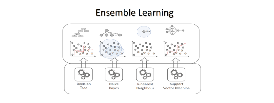
Ensemble Learning Models

For a given data set, a single algorithm may not make the best prediction. Machine learning algorithms have limitations, and creating a model with high accuracy is difficult. We can improve overall accuracy by building and combining multiple models. The combination of models is then implemented by aggregating the output from each model with two goals in mind:

• Model error reduction

• Keeping the model’s generalisation

Random Forest

A random forest is a machine learning technique for solving regression and classification problems. It makes use of ensemble learning, a technique that combines many classifiers to solve complex problems.

A random forest algorithm is made up of numerous decision trees. The random forest algorithm’s ‘forest’ is trained using bagging or bootstrap aggregation. Bagging is a meta-algorithm that improves the accuracy of machine learning algorithms through an ensemble approach.

The outcome is determined by the (random forest) algorithm based on the predictions of the decision trees. It predicts by averaging or averaging the output of various trees. The precision of the outcome improves as the number of trees increases.

Voting Classifier

The VotingClassifier combines conceptually different machine learning classifiers and predicts class labels using a majority vote or the average predicted probabilities (soft vote). A classifier of this type can be useful for balancing the individual weaknesses of a group of models that perform similarly well.

How can it be used for our dataset?

We have decided to use Weighted Average Probabilities (Soft Voting), for our Voting classifier. Soft voting returns the class label as argmax of the sum of predicted probabilities.The weights parameter can be used to assign specific weights to each classifier. When weights are supplied, the predicted class probabilities for each classifier are accumulated, multiplied by the classifier weight, and averaged. The class label with the highest average probability is then used to generate the final class label.

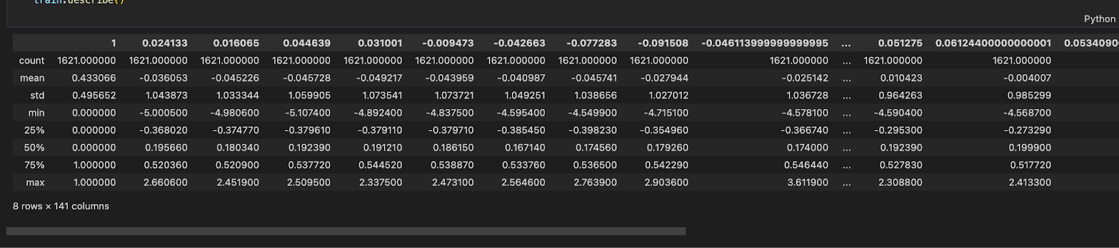
Describing the dataset

Our dataset is already standardised as seen in Figure 1.1. It has a total of 140 columns and 1621 rows. We still need to Normalize our database as Bernoulli Naïve Bayes cannot accept negative values. We have achieved this by creating a Pipeline and adding MinMaxScaler in the pipeline when we encounter the Bernoulli Naïve Bayes classifier.

classifier = Pipeline([(‘Normalizing’,MinMaxScaler()), (‘BernoulliNB’,BernoulliNB())])

Scaling converts one set of variables into another set of variables with the same order of magnitude. Because it is usually a linear transformation, it does not affect the correlation or predictive power of the features.

Why is normalising or standardizing our data necessary? It’s because the order of magnitude of the characteristics can affect the performance of some models. Some models might “believe” that one characteristic is more significant than another if, for instance, one feature has an order of magnitude equal to 1000 and another has an order of magnitude equal to 10. The order of magnitude doesn’t tell us anything about the predictive power, hence it is biased. We may eliminate this bias by changing the variables to give them the same order of magnitude.

Standardization and normalisation are two of these transformations, which convert each variable into a 0–1 interval (which transforms each variable into a 0-mean and unit variance variable). Standardisation, theoretically, is superior to normalisation because it does not cause the probability distribution of a variable to shrink in the presence of outliers

Building the Model

We have used Support Vector Machines, Bernoulli Naïve Bayes, K Nearest neighbour and Random Forest Classifier in tandem to effectively gauge the difference between all the models. For KNN, we have used different parameters of n_neighbours (1 to 25 in step 2 sizes) to find the best parameter for our classifier. GridSearchCV evaluates the model for each combination of the values passed in the dictionary using the Cross-Validation method. As a result of using this function, we can calculate the accuracy/loss for each combination of hyperparameters and select the one with the best performance.

from sklearn.model_selection import GridSearchCV
from sklearn.neighbors import KNeighborsClassifier
from sklearn.ensemble import RandomForestClassifier
from sklearn.naive_bayes import BernoulliNB
from sklearn.ensemble import RandomForestClassifier
from sklearn import svm
from sklearn.svm import SVC
import warnings
warnings.filterwarnings(‘ignore’)
from sklearn.preprocessing import MinMaxScaler
from sklearn.pipeline import Pipeline

processed_data = {}
def construct_model(dataframe):
 # the list of classifiers to use
 # use random_state for reproducibility
 classifiers = [
 SVC(probability=True, random_state=42),
 BernoulliNB(),
 KNeighborsClassifier(),
 RandomForestClassifier(random_state=42),
 ]
 
 svm_parameters = {
 ‘gamma’: [‘auto’]
 }

gaussian_parameters = {
 }

knn_parameters = {
 ‘n_neighbors’: np.arange(1, 25, 2)
 }

rf_parameters = {
 
 }
 # stores all the paramete rs in a list
 parameters = [
 svm_parameters,
 gaussian_parameters,
 knn_parameters,
 rf_parameters
 ]
 processed_data[‘estimators’] = []
 # iterate through each classifier and use GridSearchCV
 for i, classifier in enumerate(classifiers):
 if i == 1:
 classifier = Pipeline([(‘Normalizing’,MinMaxScaler()), (‘BernoulliNB’,BernoulliNB())])
 else:
 clf = GridSearchCV(classifier, # model
 param_grid = parameters[i], # hyperparameters
 scoring=’accuracy’, # metric for scoring
 cv=10,
 n_jobs=-1, error_score=’raise’)
 clf.fit(dataframe[“X_train”], dataframe[“Y_train”])
 # add the clf to the estimators list
 processed_data[‘estimators’].append((classifier.__class__.__name__, clf))

We have also built an ensemble model, specifically a Weighted Average Probabilities (Soft Voting) classifier. Soft voting returns the class label as argmax of the sum of predicted probabilities. The weights parameter can be used to assign specific weights to each classifier. When weights are supplied, the predicted class probabilities for each classifier are accumulated and multiplied by the classifier.

from sklearn.ensemble import VotingClassifier

ensemble = VotingClassifier(processed_data[‘estimators’],
 voting=’soft’,
 weights=[1,1,2,1], n_jobs=-1) # n-estimators

ensemble.fit(transformed_df_train[“X_train”], transformed_df_train[“Y_train”])

Model Evaluation

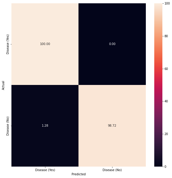
**Figure 1.2 **shows how well our last model, i.e, Ensemble Voting classifier performed and how well it approximates the relationship between having a disease and not having a disease through the use of Confusion Matrix.

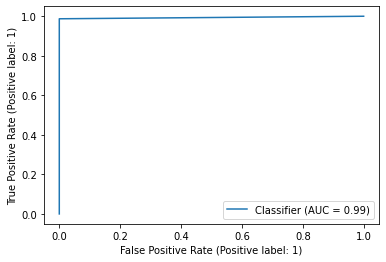
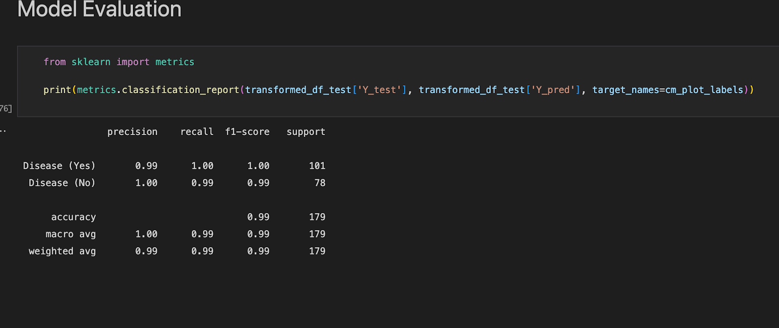
**Figure 1.3 **shows the ROC curve and **Figure 1.4 **reports the model’s performance against a range of metrics such as Precision, recall, Accuracy and F1-score.

Justification of Model Evaluation

Confusion Matrix

There are four possible outcomes here: True Positive (TP) denotes that the model predicted a true outcome and that the actual observation was true. False Positive (FP) indicates that the model predicted a true outcome but the observed result was false. False Negative (FN) indicates that the model predicted a false outcome while the observed outcome was correct. Finally, the True Negative (TN) indicates that the model predicted a false outcome while the actual outcome was also false. Our model predicts a True Positive of 100% for Disease (Yes) and a False Positive of 1.28% which is a good indicator for measuring accuracy. Subsequently True Negative is at 99.72% while True Positive is at 0%.

How do different weights in Voting Classifier affect the accuracy?

We have decided to use Weighted Average Probabilities (Soft Voting), for our Voting classifier. Soft voting returns the class label as argmax of the sum of predicted probabilities. The weights parameter can be used to assign specific weights to each classifier. When weights are supplied, the predicted class probabilities for each classifier are accumulated, multiplied by the classifier weight, and averaged. The class label with the highest average probability is then used to generate the final class label. In short, a sequence of weights is assigned for every classifier to weigh the occurrences of predicted class probabilities before an average is taken of the said weights for soft voting.

Experiment 1

Classifier: Voting Classifier

Weights: [1,1,1,1]

Observation: **Figure 1.5 **shows the confusion matrix we get with the above weights

Inference: With weights distributed evenly for all the classifiers the accuracy achieved is an average accuracy for all the ensemble classifies, i.e, an average of Support Vector Machines, Bernoulli Naïve Bayes, K Nearest neighbour and Random Forest Classifier. The average accuracy achieved is ~98.8%.

Experiment 2

Classifier: Voting Classifier

Weights: [1,1,2,1]

Observation: **Figure 1.6 **shows the confusion matrix we get with the above weights

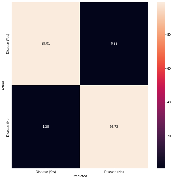
Inference: Since K Nearest neighbour had the best accuracy among all the other classifiers, we give more weight to KNN classifier. As a result, our accuracy jumps to ~99.4% which is more than the accuracy achieved in Experiment 1.

Conclusion

Ensemble Learning, Support Vector Machines, Bernoulli Nave Bayes, K Nearest Neighbor, and the Random Forest Classifier were all heavily used in the development of our Classification models. Using GridSearchCV for hyperparameter tuning and a Voting Classifier for an eventual ensemble of all the existing models, we achieved a maximum accuracy of 99.4%.

References

1. https://github.com/nandangrover/learning-models

2. https://en.wikipedia.org/wiki/Support-vector_machine

3. Hands-on Machine Learning with Scikit-Learn and Tensorflow by Aurélién Géron