Text Classification in NLP using Cross Validation and BERT
In natural language processing, text categorization tasks are common (NLP). Depending on the data they are provided, different classifiers may perform better or worse (eg. Uysal and Gunal, 2014). However, there is data where a correlation between (vectorised) texts and classes would be expected, but the assumption is not satisfied, and the classifiers perform poorly. The main reason for this is that there are a lot of classes and a lot of different texts. We’ll look at a variety of preprocessing strategies as well as techniques for improving the classifier’s performance.
In order to gain useful insights from our data we have built four classifiers:
-
Binary Classifier for predicting if a sentence was uttered by therapist or client
-
Binary Classifier for labelling if a conversation is high quality or low quality
-
Multi-Class Classifier for classifying text to appropriate behaviour type
-
Bert Transformer for classifying text to appropriate behaviour type
The folder structure for the architecture is shown in Figure 1. “binary_classifier_interlocutor.ipynb” file stores our binary classifier which uses ensemble learning to classify if a text was uttered by the therapist or the client while “binary_classifier_quality.ipynb” determines if the overall conversation between a therapist and client is of high quality or low quality. The “multi_class_classifier.ipynb” classifies the correct behaviour type for a conversation uttered by therapist and client. “transformer.ipynb” uses the BERT architecture to classify the behaviour type for a conversation uttered by therapist and client, i.e, the same result we are trying to achieve with “multi_class_classifier.ipynb”. The code can be found here: https://github.com/nandangrover/nlp-classification .
Preprocessing
Data preprocessing is an essential step in building a Machine Learning model. The primary focus for our data is limited to columns: mi_quality, topic, utterance_text, interlocutor, main_therapist_behaviour and client_talk_type. We also need to process the utterance_text column in order to reduce text dimensions.
Analysis
We do our initial exploratory analysis of the data by calculating the mean, standard deviation and 25/50/75% value on the utterance text length (Figure 2). We observe that there is a large variance in the length of text (minimum 1 word to maximum 246 words for the client). Since it’s not a translation problem we are trying to solve and also since our eventual model would not be LSTM, we have decided to not do text padding in order to make all the sentences similar in size.

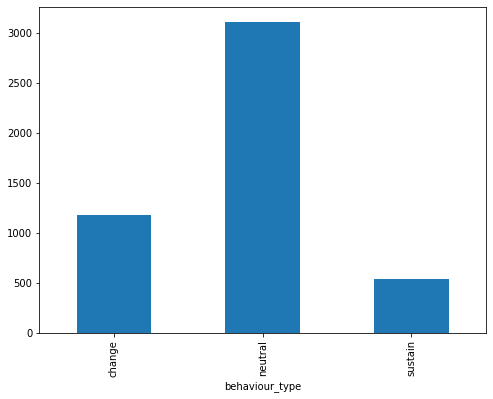
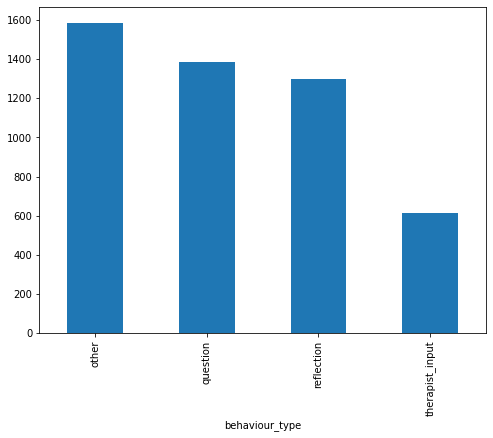
Bar charts were also created to get an idea about how the data was distributed between the different classes. Figure 3 shows the number of texts for each behaviour type for the therapist and the client.
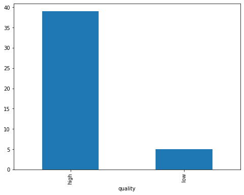
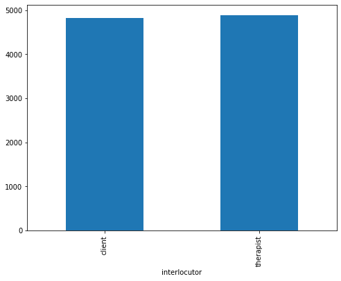
We have also analyzed our data for the binary classifier which predict the quality of texts based on the whole conversation. Figure 4 display the number of high-quality conversations vs the number of low-quality conversation. We can observe that our data has a lot more high-quality conversations than the low-quality ones. Any classifier built through this data will have an inherent bias toward high-quality conversations. Figure 4 also shows the distribution of texts between client and therapist. The binary classifier built for detecting a client talking vs the therapist talking has equal distribution in terms of utterance texts. This data shows promise for the binary classifier that will be built.
Data Cleaning
Conventional algorithms are often biased towards the dominant class, ignoring the data distribution. Minority classes are treated as outliers and neglected in the worst-case scenario [2]. For some applications, such as fraud detection or cancer prediction, we may need to configure our model carefully or artificially balance the dataset, such as by undersampling or oversampling each class. In our instance of learning unbalanced data, however, the majority of classes may be of tremendous interest. A classifier with high prediction accuracy for the majority class while preserving adequate accuracy for the minority classes is desirable. As a result, we’ll leave it alone.
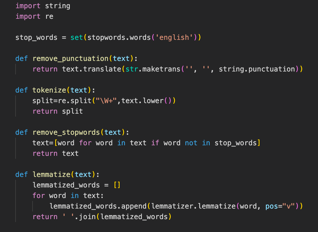
We have built similar functions for all the four classifiers to clean and enhance the utterance text. This includes removing the punctuation, tokenizing the text, removing stopwords and lemmatizing. In lemmatization, we derive the root of the word from the input words, which we have decided to choose over stemming a word. **Figure 5 **shows the methods used to perform these data preprocessing techniques.
Feature Extraction and Evaluation
Because most classifiers and learning algorithms require numerical feature vectors with a fixed size rather than raw text documents with variable length, they cannot analyse the text documents in their original form. As a result, the texts are converted to a more understandable representation during the preprocessing step.
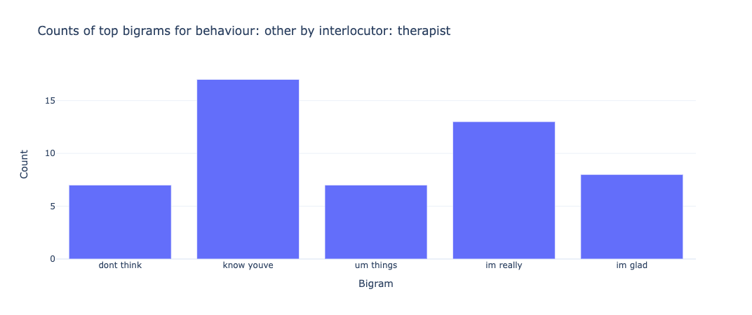
The bag of words model is a method for extracting characteristics from the text in which the presence (and often the frequency) of words is considered for each document or text in our example, but the order in which they occur is ignored. We will generate a measure called Term Frequency, Inverse Document Frequency, shortened to tf-idf for each term in our dataset. To create a tf-idf vector for each utterance text, we’ll use sklearn.feature extraction.text.TfidfVectorizer: To use a logarithmic form for frequency, set sublinear df to True. The minimal number of documents in which a word must appear to be retained is min_df, which is set to 5. To ensure that all of our feature vectors have a euclidian norm of 1, the norm is set to l2. The value of the ngram range is (1, 2), indicating that both unigrams and bigrams should be considered. To limit the number of noisy features, stop words are set to “english” to remove all common pronouns (“a,” “the,” etc.). **Figure 6 **and **Figure 7 **show the bigrams along with their count for each interlocutor.
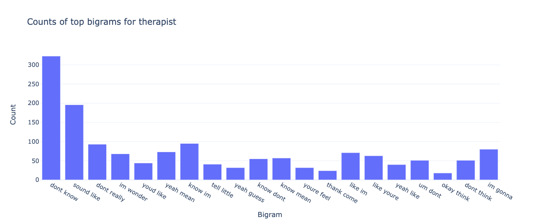
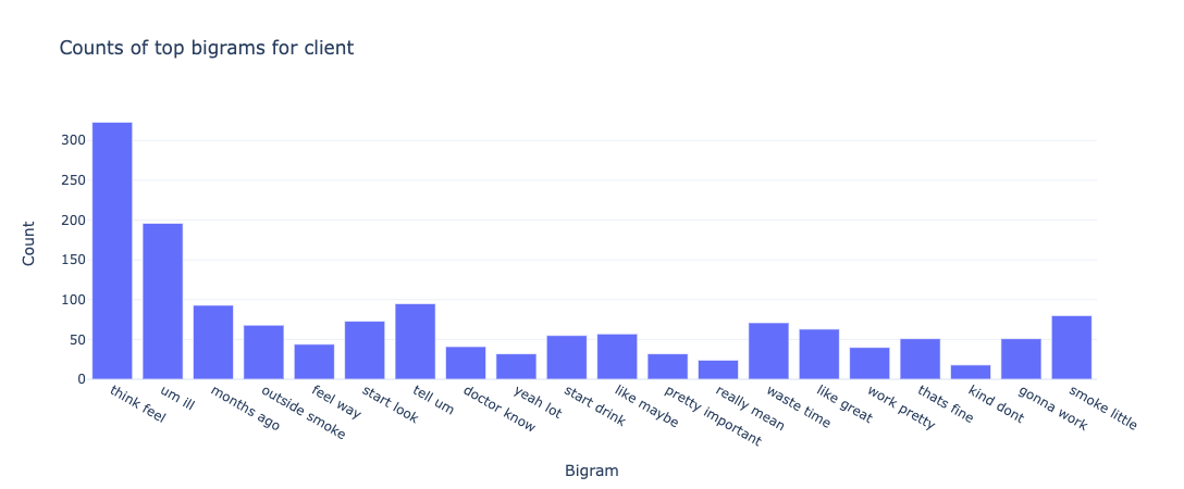
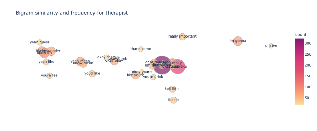
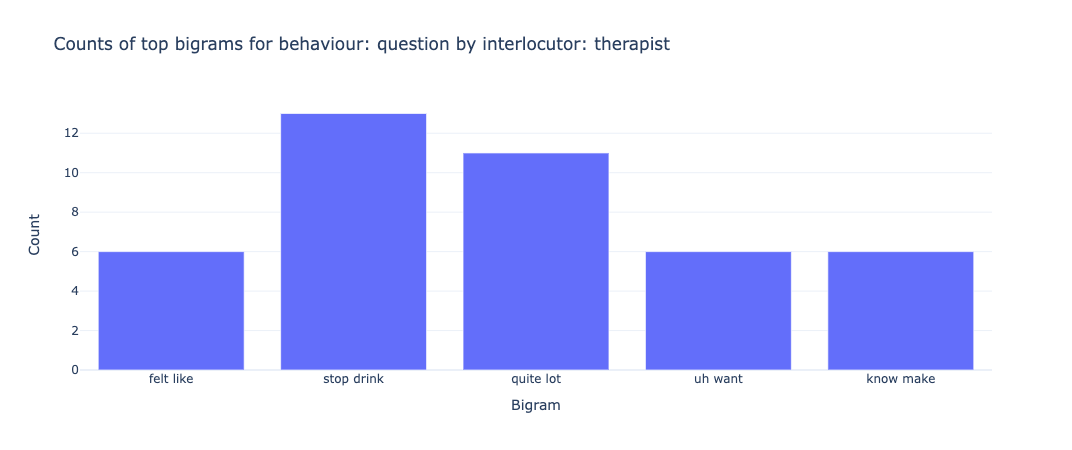
Figure 8 and Figure 9 show the bigrams along with their count for some of the behaviour types for the therapist. As we can see from the graphs for therapist and client, the bigrams are almost equal in size and distributed pretty similarly. We can sort of predict from these features that our classifier will not be biased and give pretty similar results for both classes. However, bigrams for behaviour types show an unusual amount of bigram count for type: change. We ultimately see similar results in our classifier when change is predicted incorrectly for the most amount of time and this gets a 34% f1-score. We see something similar for therapist_input class for interlocutor therapist.
Bar graphs showing the count of bigrams for each behaviour type were plotted in the code and can be seen in the Jupyter Notebook.
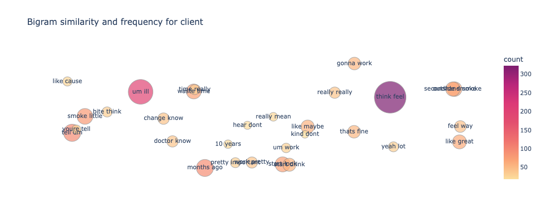
What we ultimately want to know is how these bigrams, correlate with each other in the vector space. Based on this correlation our classifiers predict which class a particular text should belong to. To visualize this correlation we make use of a bubble chart shown in Figure 10 and Figure 11. Word embeddings (specifically dense embeddings) allow for qualitative comparisons of words. They can represent words, and by extension, concepts or documents, as high-dimensional vectors, allowing for intriguing visualisations.

Using the t-SNE dimensionality reduction technique, high-dimensional bigrams are represented as two-dimensional representations.
Model Architecture
The algorithms and models used for the first three classifiers are essentially the same. We have only tweaked the preprocessing steps to get the desired input parameters. Ensemble learning proved to be effective for binary classification but through experimentation, it was found that it reduced the overall accuracy of the multi-class classifier. To this effect, we have used Logistic Regression as the final model for our evaluation. The fourth model which is also used for multi-class classification is built using the famous BERT architecture.
Binary Classifier and Multiclass Classifier
Algorithm Selection
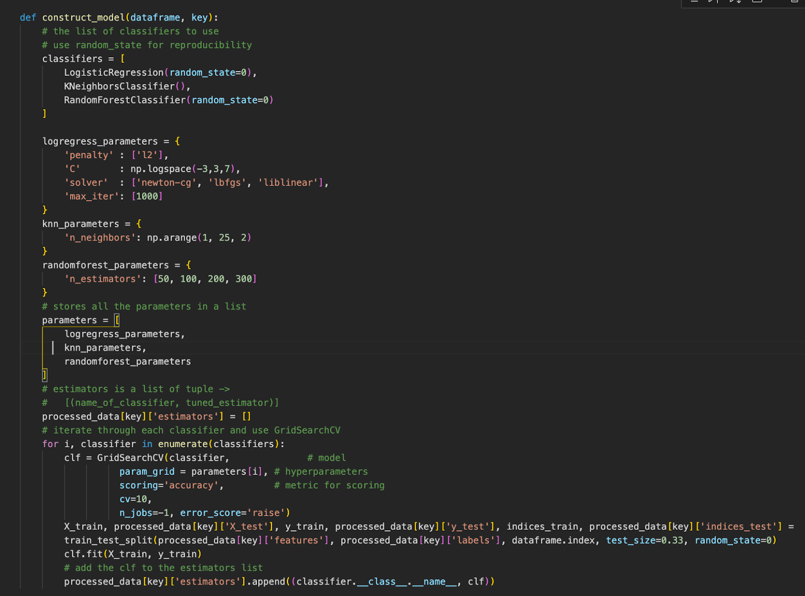
The vectorized input from “TfidfVectorizer” is used for the algorithms Logistical Regression, K-Nearest Neighbour and Random Forest (Figure 12). Some important things that were considered during these selections were:
Random Forest: The ultimate feature importance in a Random forest is the average of all decision tree feature importance. A random forest is an ensemble classifier that makes predictions using a variety of decision trees. It works by fitting a variety of decision tree classifiers to different subsamples of the dataset. In addition, each tree in the forest is made up of a random selection of the best attributes. Finally, activating these trees produces the best collection of characteristics out of all the random subsets. For many classification applications, random forest is now one of the best-performing algorithms.
K-Nearest Neighbour: The k-Nearest Neighbor algorithm has a simple concept behind it. The method seeks the k nearest neighbours among the training documents to classify a new document and uses the categories of the k nearest neighbours to weight the category candidates [3]. The kNN algorithm’s efficiency is one of its limitations, as it must compare a test document with all samples in the training set. Furthermore, the success of this technique is highly dependent on two factors: a proper similarity function and an acceptable k value.
Logistic Regression: A statistical method for binary classification that can be applied to multiclass classification is the logistic regression model, which is similar to Adaline and perceptron. Scikit-learn supports multiclass classification tasks with a highly streamlined version of logistic regression implementation [4]. Due to this reason, we are using the algorithm for both our binary classification task as well as our multiclass classification task.
Hyperparameter Tuning
GridSearchCV was used for hyperparameter tuning. Grid Search starts with defining a search space grid. The grid consists of selected hyperparameter names and values, and grid search exhaustively searches the best combination of these given values. After running the model for 10 cross-validations we got the following results for the Multi-Class Classifier (client interlocutor):
SVC Tuned Hyperparameters : {‘C’: 10, ‘gamma’: 1, ‘kernel’: ‘rbf’, ‘probability’: True} Accuracy : 0.6541670672845797 __________________________________________________________ LogisticRegression Tuned Hyperparameters : {‘C’: 1.0, ‘penalty’: ‘l2’, ‘solver’: ‘newton-cg’} Accuracy : 0.6736947868392208 __________________________________________________________ KNeighborsClassifier Tuned Hyperparameters : {‘n_neighbors’: 17} Accuracy : 0.6507605330461704 __________________________________________________________ RandomForestClassifier Tuned Hyperparameters : {‘n_estimators’: 200} Accuracy : 0.651072053535373 __________________________________________________________ The binary classifier gave the following results (classifying client): LogisticRegression Tuned Hyperparameters : {‘C’: 1.0, ‘max_iter’: 1000, ‘penalty’: ‘l2’, ‘solver’: ‘newton-cg’} Accuracy : 0.7469996444233733 __________________________________________________________ KNeighborsClassifier Tuned Hyperparameters : {‘n_neighbors’: 3} Accuracy : 0.5972587412587413 __________________________________________________________ RandomForestClassifier Tuned Hyperparameters : {‘n_estimators’: 100} Accuracy : 0.7471520682707123 __________________________________________________________
Ensemble Learning
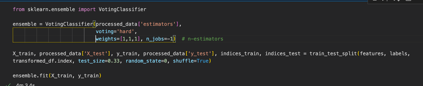
To improve generalisation performance, ensemble learning mixes numerous separate models. Deep learning models with multilayer processing architecture are now outperforming shallow or standard classification models in terms of performance [5]. Deep ensemble learning models utilise the benefits of both deep learning and ensemble learning to produce a model with improved generalisation performance. We make use of ensemble learning through a Voting Classifier to increase our model’s performance.
A Voting Classifier is a machine learning model that learns from an ensemble of models and predicts an output (class) based on the highest probability of the output being the chosen class. It simply adds up the results of each classifier supplied into the Voting Classifier and predicts the output class based on the most votes. Rather than constructing separate specialised models and determining their performance, we create a single model that trains on various models and predicts output based on the cumulative majority of votes for each output class. **Figure 13 **illustrates the parameters and weights used for our voting classifier. The estimators (weights and parameters) set during the HyperParameter Tuning are used as an input for the ensemble model.
Transformer using BERT
Recent breakthroughs in neural architectures, such as the Transformer, and the introduction of large-scale pre-trained models, such as BERT, have transformed the area of Natural Language Processing (NLP), pushing the state of the art for a variety of NLP tasks. The architecture of BERT is represented in Figure 14. We added 3 Dense Layers and one Dropout layer which randomly drops 25% of the neurons. The last Dense layer is the network’s output layer, it takes in a variable shape which can be either 4 or 3, denoting the number of classes for therapist and client. We use categorical crossentropy for loss along with sigmoid as an activation function for our model
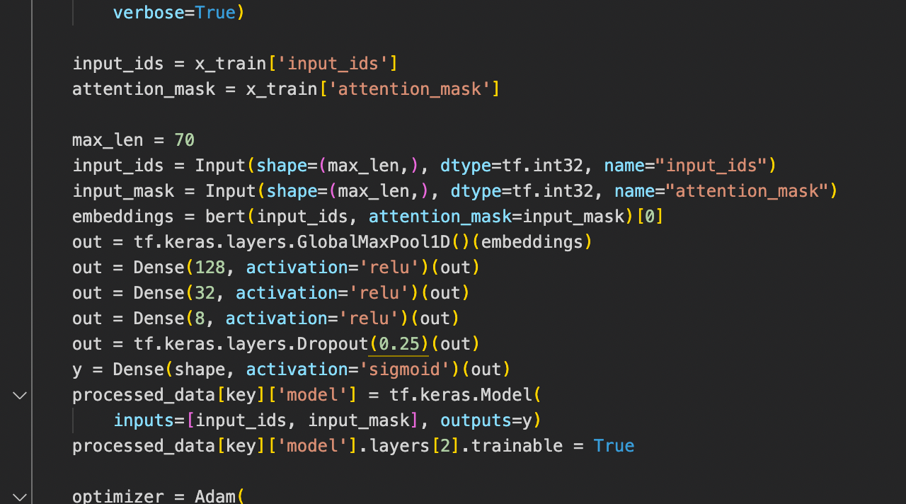
Figure 15 shows how we tracked convergence for the neural network. It is well understood that the more data a machine learning algorithm has, the more effective it may be. Even when the data is of poor quality, algorithms can outperform the original data set if the model can extract relevant information from it. Therefore, we made use of techniques such as Early Stopping and Dropout to prevent the overfitting of training data.
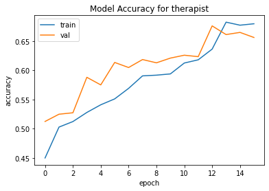
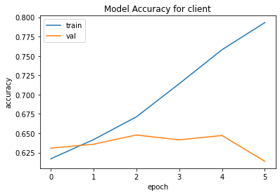
Using BERT we discovered an increase in accuracy of over 6% for classifying therapist behaviour types. The accuracy for the same model decreased by around 1% for classifying the client’s behaviour type.
Model Evaluation
We made use of multiple evaluation techniques to determine our classifier’s performance. These included building a Heatmap, listing out the wrong prediction per class and creating a Precision, Recall and F1-Score table. The following section describes in detail the performance of all the four classifiers that were built.
Heatmap
Heatmaps are coloured maps that depict data in a two-dimensional format. To display diverse details, the colour maps use hue, saturation, or brightness to achieve colour variation. The colour variation provides readers with visual information about the magnitude of quantitative numbers. Because the human brain understands pictures better than numbers, text, or other written data, HeatMaps is about substituting numbers with colours. Because humans are visual learners, displaying facts in whatever form makes greater sense. Heatmaps are visual representations of data that are simple to interpret. We use heatmaps to display relations between our different classes, i.e, behaviour types in the multi-class classifier and interlocutor in the binary classifier.
Figure 16 shows the heatmaps for predicting client and therapist behaviour types.

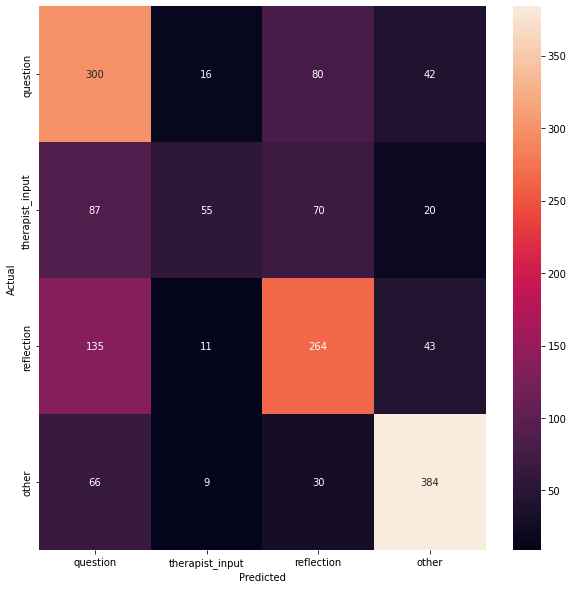
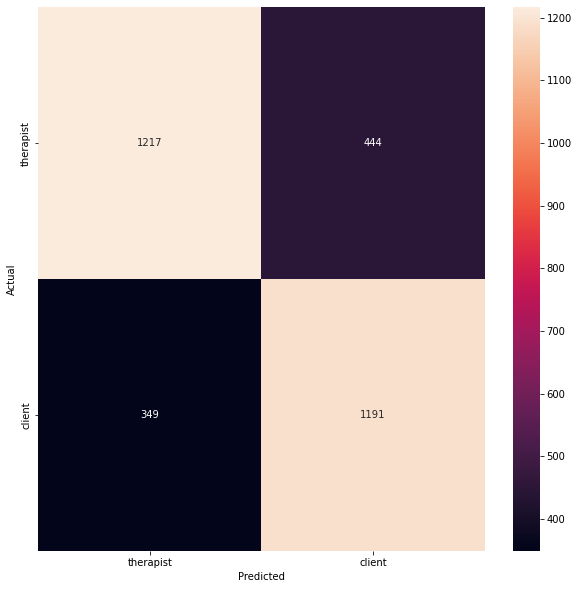
Figure 17 shows the heatmaps for predicting the interlocutor type and the quality type in the binary classifier we built. As we can see in the heatmap for quality, we have 0 texts for predicting low-quality texts. This is because the number of texts for the class “low”, which numbers at a total of 5 in our dataset.

List Wrong Predictions
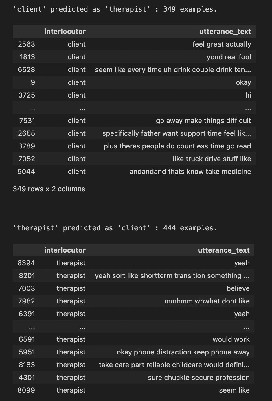
For all the classifiers built we have also listed out the wrong classifications. This helps understand the type of data which was incorrectly classified. **Figure 18 **shows the output of the misclassification code for our binary classifier.
Precision, Recall and F1-Score
Precision, Recall and F1-Score were used as the primary metric throughout the assessment to determine the quality of our model. The accuracy of the ML model indicates how many times it was correct overall. Precision refers to how well the model predicts a certain category. The recall value indicates how many times the model was successful in detecting a specific category. F1 Score is needed when we want to seek a balance between Precision and Recall.
The values for Precision, Recall and F1-Score are listed below for all the classifiers.
-
Binary Classifier for predicting if a sentence was uttered by therapist or client
precision recall f1-score supporttherapist 0.78 0.73 0.75 1661 client 0.73 0.77 0.75 1540
accuracy 0.75 3201macro avg 0.75 0.75 0.75 3201 weighted avg 0.75 0.75 0.75 3201
-
Binary Classifier for labelling if a conversation is high quality or low quality
          precision    recall  f1-score   support

     high       0.89      1.00      0.94         8
      low       0.00      0.00      0.00         1

 accuracy                           0.89         9
macro avg       0.44      0.50      0.47         9
weighted avg 0.79 0.89 0.84 9
-
Multi-Class Classifier for classifying text to appropriate behaviour type
-
Therapist
    precision    recall  f1-score   support

   question       0.51      0.68      0.58       438
therapist_input 0.60 0.24 0.34 232 reflection 0.59 0.58 0.59 453 other 0.79 0.79 0.79 489
   accuracy                           0.62      1612
  macro avg       0.62      0.57      0.57      1612
weighted avg 0.63 0.62 0.61 1612
-
Client
          precision    recall  f1-score   support

 neutral       0.68      0.93      0.78      1003
  change       0.56      0.25      0.34       403
 sustain       0.39      0.08      0.13       184

accuracy                           0.66      1590
macro avg 0.54 0.42 0.42 1590 weighted avg 0.61 0.66 0.60 1590
3. Bert Transformer for classifying text to appropriate behaviour type
-
Therapist
            precision    recall  f1-score   support

   question       0.64      0.57      0.61       438
therapist_input 0.55 0.53 0.54 232 reflection 0.58 0.68 0.63 453 other 0.88 0.83 0.85 489
  micro avg       0.68      0.68      0.68      1612
  macro avg       0.66      0.65      0.66      1612
weighted avg 0.68 0.68 0.68 1612 samples avg 0.68 0.68 0.68 1612
**2. **Client
             precision    recall  f1-score   support

     neutral       0.68      0.92      0.78      1003
      change       0.48      0.27      0.35       403
     sustain       0.00      0.00      0.00       184

   micro avg       0.65      0.65      0.65      1590
   macro avg       0.39      0.40      0.38      1590
weighted avg       0.55      0.65      0.58      1590
 samples avg       0.65      0.65      0.65      1590
Conclusion
Ensemble Learning, transformers, summarization using unigrams and bigrams and various other text pre-processing techniques were used to great effect in building our classifiers. We have reached a maximum accuracy of 75.41% for the binary classifier, 68% accuracy for predicting client behaviour types, 62% accuracy for predicting therapist behaviour types and 89% accuracy for predicting the quality of a conversation. While the amount of data available was limited, we have tried to solve the problem of generalization by using methods such as stopwords removal, tokenization, lemmatization, dropout and early stopping. Through careful data analysis and selecting appropriate algorithms for training our models, we have built multiple classifiers to correctly predict the class of an uttered text. We have also thoroughly evaluated our models through multiple metrics of evaluation.
Please do follow my page if you gained anything useful from the article. As a technical writer, every little bit helps. Cheers!
References
-
Alper Kursat Uysal and Serkan Gunal. 2014. The impact of preprocessing on text classification. Information Processing & Management, 50(1):104–112.
-
Dönicke, T., Lux, F., & Damaschk, M. (n.d.). Multiclass Text Classification on Unbalanced, Sparse and Noisy Data. https://opennlp.apache.org/docs .
-
Manning C. D. and Schutze H., 1999. Foundations of Statistical Natural Language Processing [M]. Cambridge: MIT Press.
-
Senekane, M., & Taele, B. M. (2016). Prediction of Solar Irradiation Using Quantum Support Vector Machine Learning Algorithm. Smart Grid and Renewable Energy, 07(12), 293–301. https://doi.org/10.4236/sgre.2016.712022
-
Ganaie, M. A., Hu, M., Malik, A. K., Tanveer, M., & Suganthan, P. N. (2021). Ensemble deep learning: A review. http://arxiv.org/abs/2104.02395
**BECOME a WRITER at MLearning.ai **
Related Posts
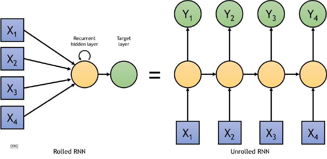
RNN for sequence-to-sequence classification
In order to understand a sequence of information we need to understand each input of data based on the understanding of previous data.
Read more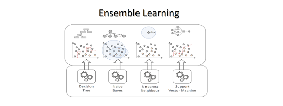
Learning based models for Classification
Thousands of learning algorithms have been developed in the field of machine learning. Scientists typically select from among these algorithms to solve specific problems.
Read more
Heart Disease Detection using fastai and sklearn
Since I began my master’s programme in artificial intelligence, I’ve been looking for a framework that will help me use my software development skills a lot more, design systems that are ready for production, and wrap some of the repetitive, everyday ML code around a framework that just works.
Read more