Convolution Neural Nets and Multi-Class Image Classification

In 2015 the idea of creating a computer system that could recognise birds was considered so outrageously challenging that it was the basis of this XKCD joke . Using fastai it’s a matter of writing a couple of lines of code to build a Convolutional Neural Network that can recognize birds with more than ~95% accuracy.

While binary classification is something we can do with a pretty good accuracy now, multi-class classification is still a little trickier. For a fixed number of training examples, binary classification is generally easier to perform than multi-class classification. As the number of classes you attempt to learn grows, so does the amount of data you must learn.

In this article, we will be building a convolutional neural net which correctly detects blood cell group from four different classes. To build this classifier we will be using a Convolution Neural Network. Due to the limited dataset available to us, we will be employing generalization techniques such as normalization, data augmentation, early stopping, and dropout to increase our model accuracy. You can find the code here: nandangrover/blood-cell-detection-cnn

Why CNN for Image Classification?

Traditional physiological trials appear to be nearly impossible to uncover because the process of pattern recognition in the brain is poorly understood. It would be a huge step forward in our understanding of the brain’s neurological mechanisms if we could create a neural network model that can recognise patterns as well as a human. In 1980, Kunihiko Fukushima published the first image classifier, Neocognitron [2], which established two types of layers in CNNs: convolutional layers and downsampling layers.

CNN has proven to be quite effective at resolving image classification problems. Many image databases, including the MNIST database, the NORB database, and the CIFAR10 dataset, have significantly improved their top performance as a result of CNN research. It is particularly good at recognising local and global structures in visual data. Simple local features such as edges and curves can be merged to produce more complex features such as corners and shapes, and finally, picture objects such as handwritten digits or human faces have obvious local and global structures. CNN has recently been used in medical imaging analysis, such as knee cartilage segmentation. [3].

In this task, we will construct a model using multiple blocks from the Convolution layer, BatchNormalization layer, and ReLU layer. Filters and Kernel Size were two parameters that were tested and tweaked to achieve the desired result. In the next section, we will talk more about why Filters and Kernel Size is so important.

Filters

The greater the number of filters, the more abstractions our Network can extract from image data. The reason for the general increase in the number of filters is that the Network receives raw pixel data at the input layer. Raw data is always noisy, and image data is especially so. As a result, we let CNN extract some relevant information from noisy, “dirty” raw pixel data first. Once the useful features have been extracted, the CNN is used to create more complex abstractions. That is why the number of filters typically increases as the Network deepens, though this is not always the case. For this reason, we are using multiple layers where the filters increase from 16 to 64.

Kernel Size

Convolutional neural networks are based on two premises:

• Localized low-level features

• What is useful in one location will be useful in another.

The size of the kernel should be determined by our level of confidence in the assumptions for the situation at hand. When we use 1x1 kernels, we effectively declare that low-level features are per-pixel, have no effect on neighbouring pixels, and should be performed on all pixels. The other extreme is kernels the size of the entire image. In this case, the CNN becomes fully connected and ceases to be a CNN, and no low-level feature locality assumptions are made. In this regard, we have selected a kernel size of 3x3 which is the default parameter selected in the case of the fastai ConvLayer method.

Data Preprocessing

Deep learning applications in medicine have a number of limitations [4]. Among these is uncertainty about the generalizability of the developed models, i.e. their ability to predict data from sources other than those used in model training [5]. Under these conditions, the model’s evaluation may result in overly optimistic assumptions about its overall performance. We use techniques like Normalization, Dropout, Data Augmentation, and Early Stopping to limit such generalisation.

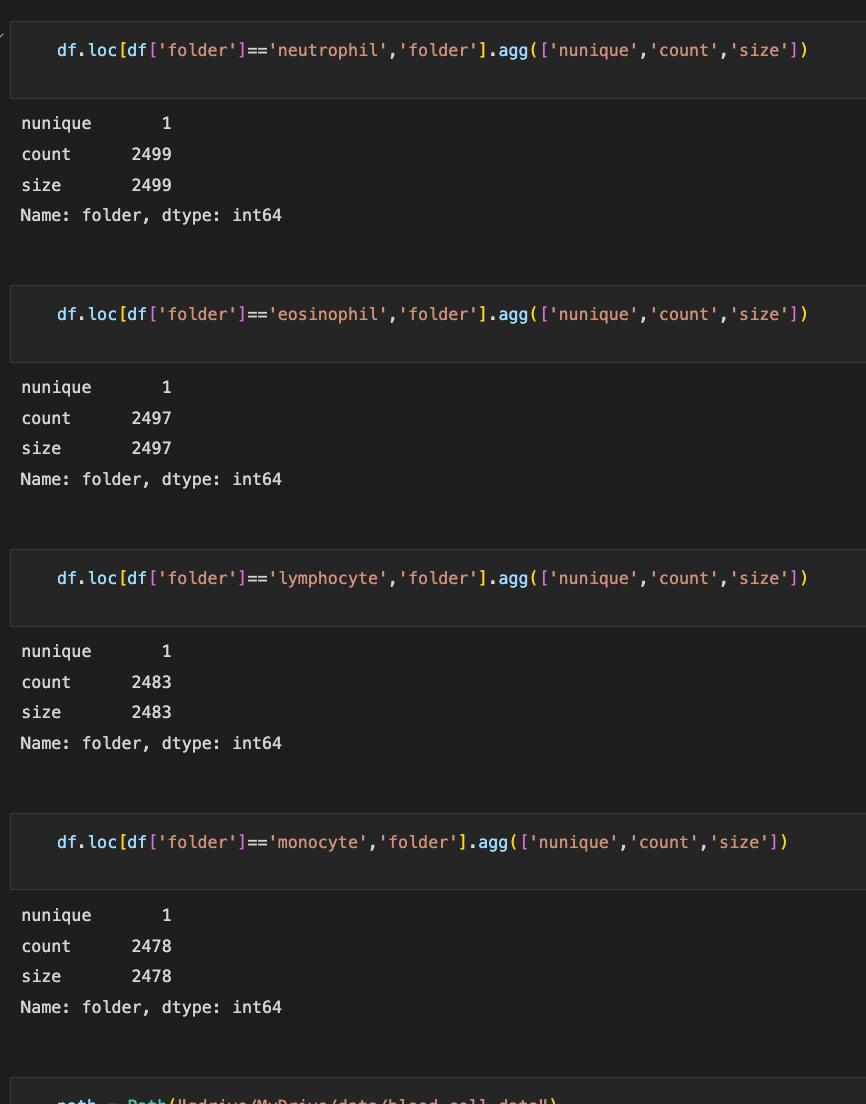
Checking for imbalanced classes

Class imbalance occurs when one class, the minority group, contains significantly fewer samples than the other class, the majority group. In many problems, the minority group is the class of interest, i.e., the positive class. Most machine learning algorithms work best when the number of samples in each class is about equal. This is because most algorithms are designed to maximize accuracy and reduce errors. Figure 2.1 shows that our dataset isn’t facing this problem and we don’t have to worry about class imbalances.

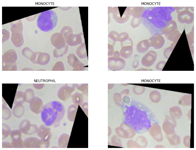
Data Augmentation and Normalization

It is well understood that the more data a machine learning algorithm has, the more effective it may be. Even when the data is of poor quality, algorithms can outperform the original data set if the model can extract relevant information from it. For our Image classifier, we have used the fastai aug_transforms method to augment the images. We have also Normalized our images. Data normalisation is an important step that ensures the data distribution of each input parameter (pixel in this case). This speeds up convergence while training the network.

batch_tfms = [ToTensor(), *aug_transforms(flip_vert=True, max_lighting=0.1, max_zoom=1.05, max_warp=0.), Normalize()]
cells = DataBlock(blocks=(ImageBlock, CategoryBlock),
 get_items=get_image_files,
 splitter=RandomSplitter(valid_pct=0.2, seed=42),
 get_y=parent_label,
 batch_tfms = batch_tfms)

dls = cells.dataloaders(path/”TRAIN”,bs=128)

Figure 2.2 shows a batch of augmented and normalized data.

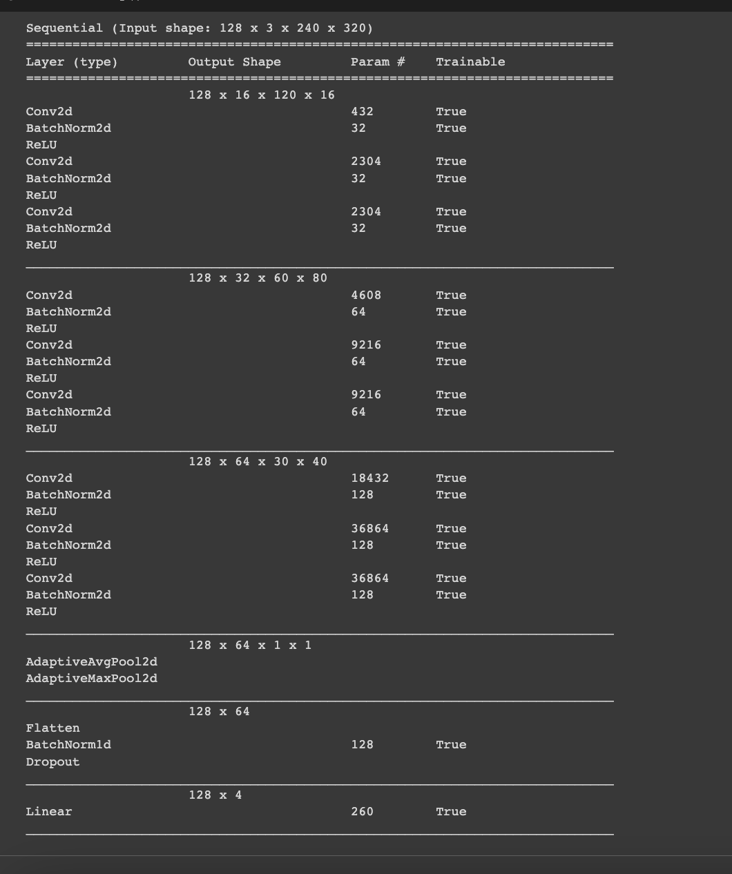
Model Architecture

The architecture of the model is shown in **Figure 2.3. **A 2-dimensional convolutional layer is the model’s initial layer. The Network receives raw pixel data at the input layer, which explains why the number of filters is generally increasing. Raw data is inherently noisy, and image data is no exception.

This layer will contain 16 output filters, each with a 3x3 kernel size, and the relu activation function will be used. Each set of layers (total of 3 sets) has a set of 3 Conv2d and 3 BatchNorm2d and also 3 ReLU activations. Batch normalisation (also known as batchnorm) works by averaging the mean and standard deviations of a layer’s activations and using those to normalise the activations. However, this can cause issues because the network may require a high number of activations in order to make accurate predictions. As a result, they added two learnable parameters, gamma and beta, which will be updated during the SGD step.

A batchnorm layer returns gamma*y + beta after normalising the activations to obtain a new activation vector y. As a result, our activations can have any mean or variance, independent of the mean and standard deviation of the previous layer’s results. These statistics are learned separately, making training our model easier. The behaviour differs between training and validation: during training, we use the batch mean and standard deviation to normalise the data, whereas, during validation, we use a running mean of the statistics calculated during training.

These layers are followed by the AdaptiveAvgPool2D layer and an AdaptiveMaxPool2D. By adding both in the final layer, we are letting Neural Net choose what works best without having to experiment ourselves. The output of the convolutional layer is then flattened and passed to a Linear layer. Because this Linear layer is the network’s output layer, it has 4 nodes, one for each class. We will use CrossEntropyLossFlat as our loss function which works best with multi class classification.

Dropout

The Dropout layer is a mask that eliminates some neurons’ contributions to the next layer while leaving all others alone. Dropout layers are useful in training CNNs because they prevent the training data from overfitting. If they are not present, the first batch of training samples has a disproportionately large influence on learning. As a result, learning of features that appear only in later samples or batches would be prevented. We are using a Dropout layer with a rate of 0.25 which results in 25% of the input units dropping. After adding dropout the accuracy increased from 91.43% to 93.6%

Early Stopping

Early stopping is an innovative method for regularising a machine learning model. It achieves this by stopping training when the validation error is at a minimum. Figure 2.3 shows our model being trained.

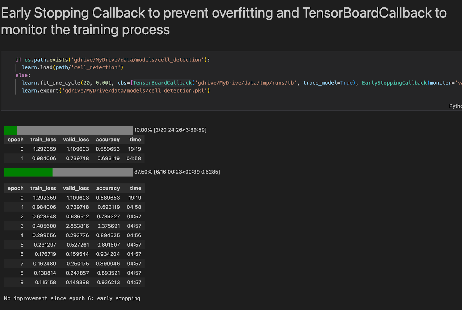
As the epochs pass, the algorithm learns, and its error on the training set, as well as its error on the validation set, decreases naturally. However, after a while, the validation error stops decreasing and begins to rise again. This indicates that the model is starting to overfit the training data. We simply stop training with Early Stopping when the validation error reaches a certain threshold.

Model Evaluation

After predicting the model’s output on test data a heat map (Figure 2.4) was created. As we can see from the results shown in the heatmap, our predictions are biased towards Neutrophil (95.83%) while the results for predicting Monocyte (75%) is the worst. While the results are not bad, they can certainly be improved by increasing the number of parameters being trained or by using state-of-the-art models, such as Resnet for our training purposes.

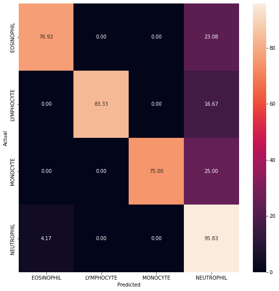
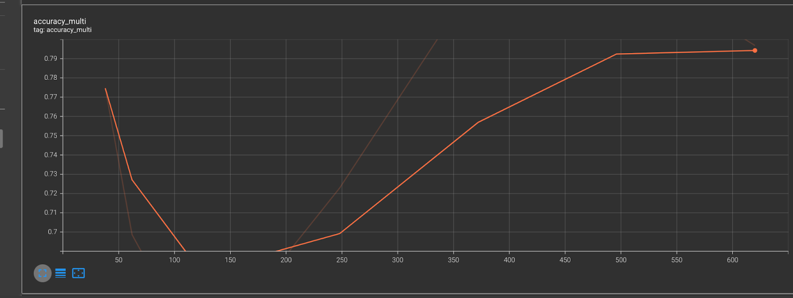
Figure 2.5 shows how our accuracy increases over every epoch.

Conclusion

Convolution Neural Networks were used to great effect in building our Neural Network. By building a custom classifier, we have reached an average multiclass accuracy of 93.62% for the CNN model. While the amount of data available was limited, we have tried to solve the problem of generalization by using methods such as Normalization, Data Augmentation, Dropout and Early Stopping. By efficiently training through a relatively small dataset, our model shows a high probability of the classification of the correct blood cell image.

References

1. Fukushima, K. (1980). Biological Cybernetics Neocognitron: A Self-organizing Neural Network Model for a Mechanism of Pattern Recognition Unaffected by Shift in Position. In Biol. Cybernetics (Vol. 36).

2. Prasoon, A., Petersen, K., Igel, C., Lauze, F., Dam, E., Nielsen, M.: Deep feature learning for knee cartilage segmentation using a triplanar convolutional neural network. in MICCAI LNCS 8150, 246–253 (2013)

3. Topol, E. J. High-performance medicine: the convergence of human and artifcial intelligence. Nat. Med. 25, 44–56. https://doi. org/10.1038/s41591–018–0300–7 (2019).

4. Krois, J., Garcia Cantu, A., Chaurasia, A., Patil, R., Chaudhari, P. K., Gaudin, R., Gehrung, S., & Schwendicke, F. (2021). Generalizability of deep learning models for dental image analysis. Scientific Reports, 11(1). https://doi.org/10.1038/s41598-021-85454-5

5. A. Halevy, P. Norvig, and F. Pereira. The unreasonable effectiveness of data. IEEE Intelligent Systems, 24(2):8–12, Mar. 2009. 1

6. Codebase: nandangrover/blood-cell-detection-cnn