Lasso Regression and Hyperparameter tuning using sklearn

Deeplearning models require high-end GPUs to be trained in a reasonable amount of time with big data, both financially and computationally. These GPUs are very expensive, but training deep networks to high performance would be impossible without them. A fast CPU, SSD storage, and fast and large RAM are all required to effectively use such high-end GPUs. Classical ML algorithms, such as Linear or Lasso regression can be trained with a decent CPU without the need for cutting-edge hardware. Because they are less computationally expensive, they allow us to iterate faster and try out more techniques in less time.

In order to explore more about regression models, we have built a body fat prediction model using Lasso regression and hyperparameter tuning. We are doing all of this while using sklearn for tasks such as data cleaning, feature engineering, data visualization and model evaluation.

What is Lasso Regression?

The Least Absolute Shrinkage and Selection Operator is abbreviated as “LASSO.” Lasso regression is a type of regularisation. It is preferred over regression methods for more precise prediction. This model makes use of shrinkage which is the process by which data values are shrunk towards a central point known as the mean. L1 regularisation is used in Lasso Regression. It is used when there are many features because it performs feature selection automatically. The main purpose of Lasso Regression is to find the coefficients that minimize the error sum of squares by applying a penalty to these coefficients.

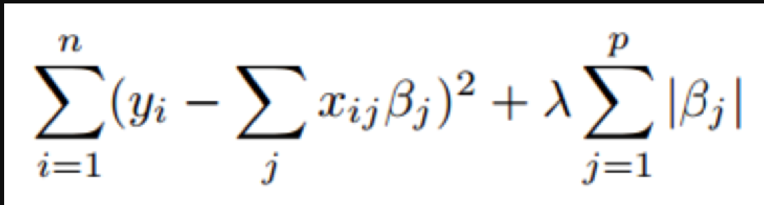
Lasso Regression Model

• λ denotes the amount of shrinkage.

• λ = 0 implies all features are considered and it is equivalent to the linear regression where only the residual sum of squares is considered to build a predictive model

• λ = ∞ implies no feature is considered i.e, as λ closes to infinity it eliminates more and more features

• The bias increases with an increase in λ

• Variance increases with a decrease in λ

Describing the dataset

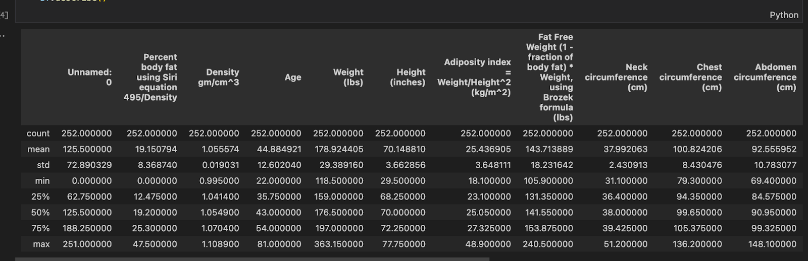
Figure 1.2 gives a brief overview of the dataset provided. The total number of features present is 18. The number of examples present is 252 and the mean body fat percentage is 19.1%. After exploring the dataset, we can see that the Unnamed: 0 columns are just used for indexing and would not be a good feature for estimating body fat, therefore it was dropped.

Data Preprocessing

Normalization is a broad term that refers to the scaling of variables. Scaling converts one set of variables into another set of variables with the same order of magnitude. Because it is usually a linear transformation, it does not affect the correlation or predictive power of the features.

Why is normalising our data necessary? It’s because the order of magnitude of the characteristics can affect the performance of some models. Some models might “believe” that one characteristic is more significant than another if, for instance, one feature has an order of magnitude equal to 1000 and another has an order of magnitude equal to 10. The order of magnitude doesn’t tell us anything about the predictive power, hence it is biased. We may eliminate this bias by changing the variables to give them the same order of magnitude.

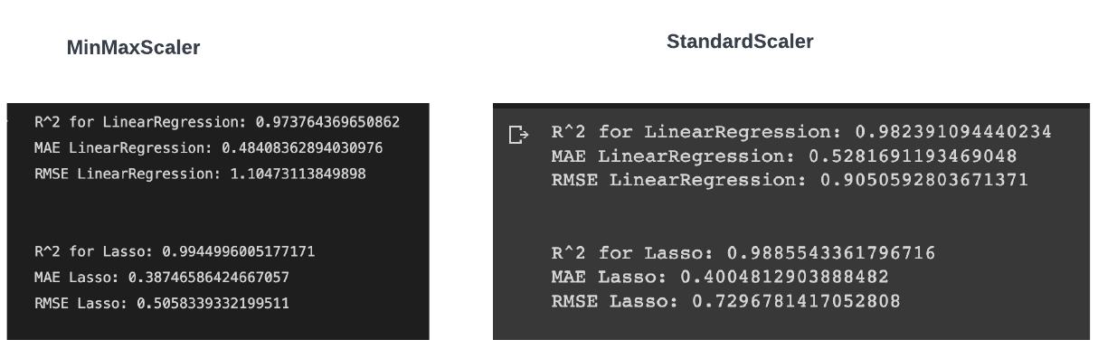
Standardization and normalisation are two of these transformations, which convert each variable into a 0–1 interval (which transforms each variable into a 0-mean and unit variance variable). Standardisation, theoretically, is superior to normalisation because it does not cause the probability distribution of a variable to shrink in the presence of outliers. But for the dataset given to us, we receive a better RMSE score using MinMaxScaler than StandardScaler which indicates a better fit. A comparison of both results is shown in Figure 1.3.

Hence for data preprocessing we have used MinMaxScaler which scales and translates each feature individually so that it falls within the training set’s given range, e.g. between zero and one. The transformation is given by:

X_std = (X — X.min(axis=0)) / (X.max(axis=0) — X.min(axis=0)) X_scaled = X_std * (max — min) + min

The code block below describes how MinMaxScaler was used to normalize our data.

from sklearn.preprocessing import MinMaxScaler
def scale_numerical(data):
 scaler = MinMaxScaler()
 data[data.columns] = scaler.fit_transform(data[data.columns])

Building the Model

We have used both Linear Regression and Lasso regression models in tandem to effectively gauge the difference between both the models. For Lasso regression, we have used 100 alpha parameters and fed them to GridSearchCV for hyperparameter tuning.

from sklearn.linear_model import Lasso, LinearRegression, LogisticRegression
from sklearn.model_selection import train_test_split
from sklearn.model_selection import GridSearchCV
from sklearn.metrics import mean_absolute_error,r2_score,mean_squared_error

def construct_model():
 # the list of classifiers to use
 regression_models = [
 LinearRegression(),
 Lasso(),
 ]

linear_model_parameters = {}

lasso_parameters = {
 ‘alpha’: np.arange(0.00, 1.0, 0.01)
 }

parameters = [
 linear_model_parameters,
 lasso_parameters
 ]

data[‘estimators’] = []

# iterate through each classifier and use GridSearchCV
 for I, regressor in enumerate(regression_models):
   clf = GridSearchCV(regressor, # model
     param_grid = parameters[i], # hyperparameters
     scoring=’neg_mean_absolute_error’, # metric for scoring
     cv=10,
     n_jobs=-1, error_score=’raise’, verbose=3)
   clf.fit(X_train, y_train)
   # add the clf to the estimators list
   data[‘estimators’].append((regressor.__class__.__name__, clf))

Cross Validation and GridSearchCV

Cross-validation is a statistical method for estimating machine learning model performance (or accuracy). It is used to prevent overfitting in a predictive model, especially when the amount of data available is limited. Cross-validation involves dividing the data into a fixed number of folds (or partitions), running the analysis on each fold, and then averaging the overall error estimate.

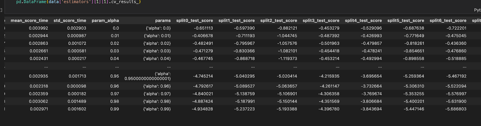
GridSearchCV evaluates the model for each combination of the values passed in the dictionary using the Cross-Validation method. As a result of using this function, we can calculate the accuracy/loss for each combination of hyperparameters and select the one with the best performance. For our model, the best value for the alpha parameter was chosen to be 0.01, which gives us a mean test score of -0.560748 and a subsequent rank of 1. The parametric score of the hyperparameter is described in Figure 1.4.

Model Evaluation

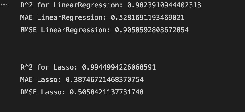
**Figure 1.5 **shows how well our model performed and how well it approximates the relationship between the actual body fat percentage and the predicted body fat percentage. We have used R2, MAE and RMSE for our evaluation.

Mean Absolute Error (MAE)

This is simply the average of the absolute difference between the target and predicted values. It’s not recommended when outliers are prominent. As we can see from our metrics the MAE error for the Lasso regressor is 0.38.

R-squared or Coefficient of Determination

This metric represents the proportion of the dependent variable’s variance that can be explained by the model’s independent variables. It assesses the strength of our model’s relationship with the dependent variable. Our Lasso regressor gives a score of 0.99 which means the model represents the variance of the dependent variable.

Root Mean Squared Error (RMSE)

The root of the average of squared residuals is what RMSE is. We know that residuals indicate how far the points are from the regression line. As a result, RMSE quantifies the scatter of these residuals. Our Lasso regressor gives a score of 0.50 showing that the model can relatively predict the data accurately.

Feature Importance

The code block below shows how we can calculate and plot the most important features used by our Lasso regression model.

import matplotlib.pyplot as plt
from textwrap import wrap

def rf_feat_importance(model, df):
 importance = model.coef_
 keys = list(df.keys())
 # summarize feature importance
 for i,v in enumerate(importance):
 print(‘Feature: %s, Score: %.5f’ % (keys[i],v))
 labels =[x[:10] for x in keys]
 fig = plt.figure()
 ax = fig.add_axes([0,0,1,1])
 ax.bar([x for x in range(len(importance))], height=importance, color=’b’)
 ax.set_xticklabels([labels[i — 1] for i in range(len(importance) +1)], rotation=45)

plt.show()
 return importance

Figure 1.6 shows the plot of our model before and after removing the low importance features.

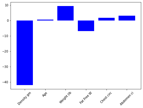
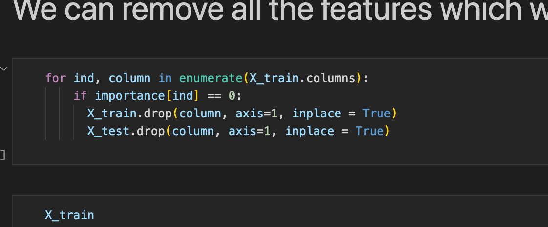
By eliminating the factors of low value, it appears plausible that we might employ just a portion of the columns and still achieve good results. So we have gone ahead and removed all the features with the importance of 0 (Figure 1.7).

This leaves us with 5 columns:

• Density gm/cm³

• Age

• Weight (lbs)

• Fat Free Weight (1 — fraction of body fat) * Weight, using Brozek formula (lbs)

• Chest circumference (cm)

• Abdomen circumference (cm)

We can conclude with a high probability that the above measurements are the most essential for calculating body fat percentage.

Conclusion

Lasso regression was used extensively in the development of our Regression model. We achieved an R-squared score of 0.99 by using GridSearchCV for hyperparameter tuning. Normalization with MinMaxScaler had a significant impact on reducing bias and increasing variance in our model. We also used model coefficients to determine the most important features required for calculating body fat percentage.

References

• Codebase: nandangrover/lasso-regression

• https://www.statisticshowto.com/lasso-regression/