A Deep Dive into Reinforcement Learning: Q-Learning and Deep Q-Learning on a 10x10 FrozenLake Environment
Reinforcement Learning is a machine learning method in which an algorithm makes decisions and takes actions within a given environment and learns what appropriate decisions to make through trial-and-error actions. Before being united in the research in the 1990s, the academic discourse for Reinforcement Learning pursued three concurrent ‘threads’ of research (trial and error, optimal control, and temporal difference). Reinforcement Learning was then able to master the games of Chess, Go, and a plethora of electronic games. Modern Reinforcement Learning applications enable businesses to optimize, control, and monitor their respective processes with incredible accuracy and finesse. As a result, the future of Reinforcement Learning is both exciting and fascinating, as research is being conducted to improve the algorithm’s interpretability, accountability, and trustworthiness.
In this blog, we will be solving the FrozenLake v1 environment problem for 10*10 state space through the use of Q-Learning and Deep Q-Learning. All the code can be found in this repository: nandangrover/reinforcement_frozenlake . The code for the Neural Network, i.e, Deep Q-Learning is stored in **deep_q_learning.ipynb **and the code for the Q-Learning method in which the agent knows about the reward at the end of the board are stored in q_learning.ipynb. Please follow the instructions in the README.md file for setting up the environment locally.
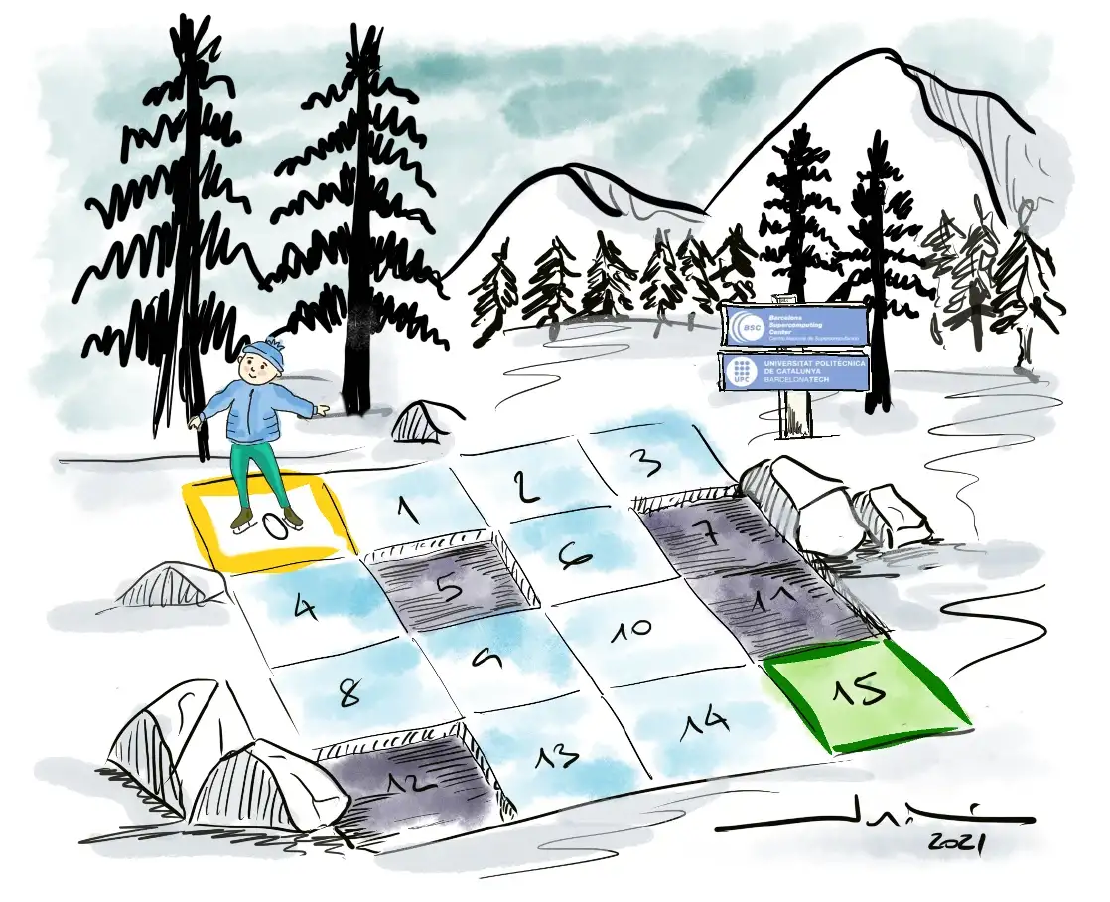
Frozen Lake Environment
Frozen Lake is a simple tile-based environment in which the AI must move from an initial tile to a goal. Tiles can be a frozen lake or a hole that keeps you stuck indefinitely. The AI, or agent, can take four different actions: LEFT, DOWN, RIGHT, or UP. To reach the goal in the fewest number of actions, the agent must learn to avoid holes. The environment is always configured the same way by default. We are not going to be using the default environment state for our task, instead, we will be using the generate_random_map method to generate a random 10*10 grid with a 0.3% probability of a frozen tile.
Environment Parameters
The game or task at hand is encapsulated by the environment. It will perform an action and then return to an object. This object contains information about the current state of the game, the reward, the discount, and whether it is a beginning, middle, or end step. The agent will operate in the environment, observe the state, and take action in accordance with its policy. It has an internal state which is trained using reinforcement learning.
The complexity of the 10*10 Board
For a 4*4 FrozenLake, the probability that a random action sequence reaches the end is at WORST 1/(4⁶) or 1/4096 for a 4x4 grid because it needs to take 3 steps right and 3 steps down. I say at worst because there are combinations of 3 right, and 3 down steps that also reach the end, but in a randomly generated frozen lake, we cannot be certain of the exact probability.
Compare this to a 10x10 frozen lake. We would need to take 9 steps right and 9 steps down at worst, which comes out to 1/(4¹⁸) or 1/68719476736. This is 4¹⁰ times or 10,48,576 times more unlikely. The is_slippery parameter makes the problem significantly harder for a 10* 10 board. In the slippery variant, the action the agent takes only has a 33% chance of succeeding. In case of failure, one of the three other actions is randomly taken instead. This feature adds a lot of randomness to the training, which makes things more difficult for our agent
Observations, State Space and Action Space
In the simplest incarnation, there is a lake with 4×4 tiles. 10*10 is bigger with a state space of 100 tiles resulting in a much higher level of randomness to the agent’s movement.
SFFF
FHFH
FFFH
HFFG
These symbols mean the following:
Actions space is defined by four numbers: 0, 1, 2, 3, 4. In the source code, we can find a mapping from direction to numbers (shown below). These actions can be taken by the agent to explore the environment. Since the is_slippery parameter is false, there is only a 33% probability that the agent will move in the direction specified by us.
Reward
The agent is only rewarded in Frozen Lake when it reaches the state G. We have no control over this reward; it is determined by the environment and is set to 1 when the agent reaches G and 0 otherwise.
Info Dictionary
Info contains information about the likelihood of the current action taken by the agent. Because we set the slippery parameter to true, the info dictionary always contains the 0.33% value, which is never used during our task.
Episode
One episode is defined as follows:
-
The agent will start with a new environment. Then it will look at the current state and derive an action using the algorithm.
-
It will tell the environment about the action and the former will perform the latter and it will result in a new state.
-
This transition is evaluated and used to update other dependent values. Once the episode has finished, the environment will automatically start anew.
Deep Q-Learning
The idea behind going deep in reinforcement learning is that the q-table becomes too large due to a large amount of state information involved. Consider the state space of a large problem. Assume we want to find the best path for delivering packets. We could use a skewed area of 128 128 fields. We might have to collect and deliver 20 packets. This results in a state space of 128x128x20x20 = 6.553.600. We would imply the following actions: left, up, right, and down. This would yield a q-table containing 6.553.600 x 4 = 26.214.400 entries. This table is no longer storable in memory for larger problems. The concept behind deep q-learning is to combine deep neural networks with reinforcement learning.
Architecture
Our neural network is built of three main components: An agent, a Buffer and a set of Sequential layers. The main function controls the execution of Agent through 10,000 episode which took roughly 3 hours to execute in a CPU.
Layers
Our model consists of one input Dense layer, a relu activation function and another output Dense layer. This layer helps in changing the dimensionality of the output from the preceding layer so that the model can easily define the relationship between the values of the data in which the model is working. In this problem, we know that the Q-table can be constructed explicitly with a 100×4 table. Choosing the output size of the layer as 4 directly gives us a single layer with predicted action.
def build_nn(num_acts, num_states=1, lr=0.001):
 model = Sequential([Dense(256, input_shape=(num_states,)),
 Activation("relu"),
 Dense(num_acts)])
 model.compile(optimizer=Adam(learning_rate=lr), loss="mse")
 return modelpyt
Agent
Our agent is the brain of the neural network. It holds the logic behind the Epsilon-Greedy algorithm as well as the calls to the neural network for action prediction. The Q-Learning algorithm is also wrapped up in this class.
The epsilon-greedy algorithm is a simple but extremely efficient method to find a good tradeoff between exploration and exploitation. Every time the agent has to take an action, it has a probability ε of choosing a random one, and a probability 1-ε of choosing the one with the highest value. We can decrease the value of epsilon at the end of each episode by a fixed amount (linear decay), or based on the current value of epsilon (exponential decay). We are using exponential delay in our architecture.
class Agent:
 def __init__(self, num_acts):
 self.num_acts = num_acts
 # self.exploration_rate = .99 # eps
 # self.exploration_decay_rate = 0.999 # eps decay
 # self.min_exploration_rate = .001 # eps min
 self.discount_rate= .95 # discount factor

 self.exploration_rate = 1
 self.max_exploration_rate = 1
 self.min_exploration_rate = 0.001
 self.exploration_decay_rate = 0.005

 self.eval_nn = build_nn(num_acts)
 self.target_nn = build_nn(num_acts)

 def choose(self, state):
 if random.random() < self.exploration_rate:
 return random.randint(0, self.num_acts - 1)

 return np.argmax(self.eval_nn.predict(np.array([state]), verbose=0))
 def learn(self, batch_size=69, game_num=0):
 buff_len = len(Buffer.action)
 if batch_size < buff_len:
 action, \
 curr_state, \
 next_state, \
 reward, \
 done = Buffer.get_sample()

 eval_q = self.eval_nn.predict(np.array(next_state), verbose=0)
 next_q = self.target_nn.predict(np.array(next_state), verbose=0)
 target_q = self.target_nn.predict(np.array(curr_state), verbose=0)
 for i in range(len(target_q)):
 max_i = np.argmax(eval_q[i])
 term = 1 - done[i]
 target_q[i][action[i]] = reward[i] + self.discount_rate * next_q[i][max_i] * term
 self.eval_nn.fit(np.array(curr_state), target_q, verbose=0)

 if buff_len % 100 == 0:
 self.target_nn.set_weights(self.eval_nn.get_weights())

 self.exploration_rate = self.min_exploration_rate + \
 (self.max_exploration_rate - self.min_exploration_rate) * np.exp(-self.exploration_decay_rate*game_num)
 exploration_rate_tracker.append(self.exploration_rate)
Buffer
The training process needs someplace to store the plays of the game. The agent will play the game in the first phase, and then will be trained on that experience. This is the feedback mechanism which will make the agent play better next time. Our Buffer holds values of 69 episodes before the values are passed to the neural network. After that, a random sample of 20 episodes is sampled, processed and fed into the q-table.
class Buffer:
   curr_state = []
   next_state = []
   action = []
   reward = []
   done = []

   def save(action, curr_state, next_state, reward, done):
       Buffer.action.append(action)
       Buffer.curr_state.append(curr_state)
       Buffer.next_state.append(next_state)
       Buffer.reward.append(reward)
       Buffer.done.append(done)

   def get_sample(num_sample=20):
       ids = random.sample(range(0, len(Buffer.action) - 1), num_sample)

       action = []
       curr_state = []
       next_state = []
       reward = []
       done = []
       for i in random.sample(range(0, len(Buffer.action) - 1), num_sample):
           action.append(Buffer.action[i])
           curr_state.append(Buffer.curr_state[i])
           next_state.append(Buffer.next_state[i])
           reward.append(Buffer.reward[i])
           done.append(Buffer.done[i])

       return action, curr_state, next_state, reward, done
Main Function
We take the following steps to run our Deep Q-learning based model:
1. Creates a new agent with 4 actions (left, right, top, bottom)
2. Creates an empty list that will hold rewards for each episode
3. Creates an empty list that will hold the exploration rate for each episode
4. For each episode (i.e., for each game):
  1. Reset the environment
  2. Set the done flag to False
  3. Set the total reward for the episode to 0
  4. For each step in the episode:
    1. Choose an action using the agent's choose function
    2. Take the action and observe the next state, reward, and done flag
    3. Save the action, current state, next state, reward, and done flag to the Buffer
    4. Have the agent learn from Buffer
5. If the done flag is True, break out of the loop
5. Append the total reward for the episode to the list of rewards
5. Plot the exploration rate over time
6. Plot the rewards over time

def main(num_games=10000, max_steps=800, mult = 1000):
   agent = Agent(env.action_space.n)
   rewards_all_episodes = []

   wins = 0.0
   for i in range(num_games):
       print("Game:", i, "Wins:", wins)
       done = False
       curr_state = env.reset()
       steps = 0
       tot_reward = 0
       while not done:
           if steps > max_steps:
               raise Exception("Too many steps")
           steps += 1

           act = agent.choose(curr_state)
           next_state, reward, done, truncated, info = env.step(act)

           wins += reward

           if not done and reward == 0 and next_state != curr_state:
             reward = 0.1 * next_state/100
           if done and reward == 0:
             reward = -0.1 * next_state/100
           if done and reward == 1.0:
             reward = 20

           done = done
           tot_reward += reward

           temp_reward = reward
           Buffer.save(act, curr_state, next_state, reward, done)
           agent.learn(69, i)
       rewards_all_episodes.append(tot_reward)
   print("Score over time: " +  str(sum(rewards_all_episodes)/num_games))
   save_model(agent)
   plot_epsilon(exploration_rate_tracker)
   plot_rewards(rewards_all_episodes, num_games, mult)
Discount adjustment
The adjustment of the discount was critical. The environment has set it to 1.0 for some reason. This means that once the agent has completed the goal, all of the steps that led to it receive a reward of 1. This means that all of the steps taken up to that point will be reinforced. We have no idea whether it moved in a straight line from start to finish or took a lot of unnecessary steps. It could have gone around the middle hole a couple of times before finishing. All of these activities would be encouraged. It would fail to reach the goal quickly if enough silly movements were encouraged. Setting the discount to 0.95 concentrates the reward on the last steps taken by the agent. It will also encourage taking a short path from beginning to end.
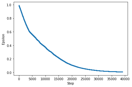
Epsilon Decay
As we can see in the figure below, the epsilon reduces till about 2000 steps and then it levels off for the next 2000 steps. At this point, the agent will stop exploring and start exploiting the environment through the use of q-values.
Rewards Progression
Due to the problem being extremely complex, we couldn’t get the agent to the chest in a reasonable amount of time and episodes. We attempted 10,000 episodes which ran for about 3 hours in Google Collab. In order to keep track of rewards progression over time, we instead made use of negative rewards and positive rewards for every time the agent dies and every time the agent survives simultaneously.
There are three main types of rewards: extrinsic rewards, intrinsic rewards, and shaped rewards. Extrinsic rewards are externally provided rewards such as money, points, or something else that is valuable. Intrinsic rewards are generated by the agents themselves based on their internal state and their own model of the environment. Shaped rewards are a combination of extrinsic and intrinsic rewards that have been designed to encourage specific types of behaviour. These distinctions come from the field of psychology but have a role in RL problems too. In our problem, we used Shaped rewards to encourage our agents to survive in this harsh environment for a longer period of time.
The figure below shows the rewards progression over time for the agent. As we can see, there are a lot of sharp downward curves in the linear graph, but the general trend of rewards over time is positive.
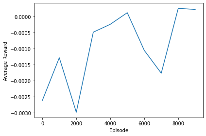
Please note, the figure above represents the **shaped rewards **given by us and not the environment itself.
Q-Learning
Q-learning is a reinforcement learning algorithm that does not require a model. It is a learning algorithm that is based on values. Value-based algorithms use an equation to update the value function (particularly Bellman equation). The other type, policy-based estimation, estimates the value function with a greedy policy obtained from the most recent policy improvement.
Q-learning is an unauthorised learner. That is, it learns the optimal policy’s value independently of the agent’s actions. An on-policy learner, on the other hand, learns the value of the policy being carried out by the agent, including the exploration steps, and it will find an optimal policy that takes into account the exploration inherent in the policy.
Figure 1.3 shows the formula for q-learning, where Q(G-1, aₜ) = 0 and maxₐQ(G, a) = 0 because the Q-table is empty, and rₜ = 1 because we get the only reward in this environment. We obtain Q{new}(G-1, aₜ) = 1. The next time the agent is in a state next to this one (G-2), we update it too using the formula and get the same result: Q{new}(G-2, aₜ) = 1. In the end, we backpropagate the ones in the Q-table from G to S.

α is the learning rate (between 0 and 1), which is how much we should change the original Q(sₜ, aₜ) value. If α = 0, the value never changes, but if α = 1, the value changes extremely fast. In our attempt, we limited the learning rate to α = 0.8.
γ is the discount factor (between 0 and 1), which determines how much the agent cares about future rewards compared to immediate ones. If γ = 0, the agent only focuses on immediate rewards, but if γ = 1, any potential future reward has the same value as current ones. In Frozen Lake, by setting the discount to 0.95, the reward will become concentrated on the last steps that the agent did. It will also encourage taking a short path from start to finish. With that in place, the whole training becomes much more focused and stable.
Architecture
As mentioned in the Rewards Progression section of the Deep Q-Learning, there are three main types of rewards: extrinsic rewards, intrinsic rewards, and shaped rewards. We will be using shaped rewards along with purposely filling the Q-table with default values based on the assumption that the reward is at the rightmost corner of the environment.
Hyperparameter Defaults
The hyperparameter defaults used in the Q-Learning algorithms (both with and without prior knowledge) are described below:
-
total_episodes: Number of episodes that the agent can play
-
learning_rate: It is the learning rate of the algorithm. It is used to update the Q-table. We have limited it to 0.8
-
max_steps: This is the maximum number of steps that the agent can take in an episode. This is used to avoid infinite loops. A general rule of thumb for to calculate the number of steps is to use this calculation: Number of actions _ State space _ 2. For our 10* 10 board, this comes out to 4 * 100 * 2 = 800 steps.
-
gamma: This is the discount factor. It is used to calculate discounted future rewards.
-
epsilon: This is the exploration rate. It is used to explore the environment.
-
max_epsilon: This is the maximum exploration rate. It is used to set the exploration rate to the maximum value.
-
min_epsilon: This is the minimum exploration rate. It is used to set the exploration rate to the minimum value.
-
decay_rate: This is the exponential decay rate of the exploration rate. It is used to decrease the exploration rate as the agent learns.
-
q_table: This is the Q-table. It is a matrix of size (state_space_size, action_space_size). It is used to store the Q-values.
total_episodes = 3000000 learning_rate = 0.8 max_steps = 800 gamma = 0.95 epsilon = 1.0 max_epsilon = 1.0 min_epsilon = 0.001 decay_rate = 0.000005 q_table = np.zeros((state_space_size, action_space_size))
Q-learning without prior knowledge of goal
In the code below, we have demonstrated how a normal q-learning algorithm will run without any foreknowledge of the goal at the rightmost tile of the environment. The q-table is updated after each step in the episode. We begin each episode by resetting the environment and initialising the state, step, done, and total rewards variables. We then enter the loop and take a step for each of the max steps. After that, we’ll decide whether to exploit or explore. We will exploit if the random number is greater than the epsilon value. If it is less, we will investigate. We then use the action to take a step into the environment. Using the Q-Learning formula, we update the q table. The total rewards and state are then updated. We exit the loop if we have reached the terminal state. The epsilon value is then updated at the end of each episode.
for episode in range(total_episodes):
 state = env.reset()
 step = 0
 done = False
 total_rewards = 0

 for step in range(max_steps):
   exp_exp_tradeoff = random.uniform(0, 1)
   if exp_exp_tradeoff > epsilon:
     action = np.argmax(q_table[state,:])
   else:
     action = env.action_space.sample()
     new_state, reward, done, info = env.step(action)
     temp_reward = reward
   q_table[state, action] = q_table[state, action] + learning_rate * (temp_reward + gamma * np.max(q_table[new_state, :]) - q_table[state, action])

   total_rewards += reward
   state = new_state

   if done == True:
     break
 epsilon = min_epsilon + (max_epsilon - min_epsilon)*np.exp(-decay_rate*episode)
 rewards.append(total_rewards)
 exploration_rate_tracker.append(epsilon)
Epsilon Decay
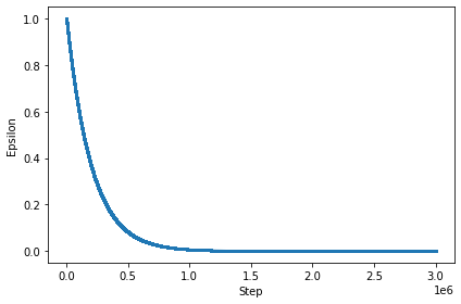
As we can see in the figure below, the epsilon reduces to about 1 million steps and then it levels off for the next 3 million steps. At this point, the agent will stop exploring and start exploiting the environment through the use of q-values.

Rewards Progression
The figure below shows the rewards progression over time for the agent who didn’t have prior knowledge of the goal at the rightmost corner. As we can see, the agent never received the reward from the environment.
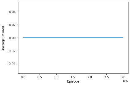
Please note, the figure above represents the **intrinsic rewards **given by the environment. Shaped rewards were not used to generate this figure.
Q-learning with prior knowledge of goal
The code below shows how a q-learning algorithm with a few tweaks can perform better than the standard q-learning algorithm which relies on randomly exploring the environment. We will be making use of **shaped rewards **as well as initializing the q-table with foreknowledge of where the goal is.
rewards = []
exploration_rate_tracker = []
# Let agent know that goal is in the right most corner


for episode in range(total_episodes):
   state = env.reset()
   step = 0
   done = False
   total_rewards = 0

   for step in range(max_steps):
       exp_exp_tradeoff = random.uniform(0, 1)
       if exp_exp_tradeoff > epsilon:
           # action = np.argmax(q_table[state,:])
           action = np.argmax(q_table[state,:])
       else:
           action = env.action_space.sample()

       new_state, reward, done, info = env.step(action)
       temp_reward = reward
       if not done and reward == 0.0 and new_state != state:
           temp_reward = 0.1 * new_state/100
       if done and reward == 0.0:
           # negative reward for falling in a hole in early states
           temp_reward = -0.1 * new_state/100
       if done and reward == 1.0:
           temp_reward = 50

       q_table[state, action] = q_table[state, action] + learning_rate * (temp_reward + gamma * np.max(q_table[new_state, :]) - q_table[state, action])

       total_rewards += reward
       state = new_state

       if done == True:
           break
   epsilon = min_epsilon + (max_epsilon - min_epsilon)*np.exp(-decay_rate*episode)
   rewards.append(total_rewards)
   exploration_rate_tracker.append(epsilon)
Q-table initialization
First, the agent must determine the location of the goal. We populate the q table with ascending values to the goal because it is in the rightmost corner. To encourage the agent to go down, we give the second index the highest value. To encourage the agent to go right, we give the third index the second-highest value. To discourage the agent from going up or left, we assign the lowest value to the other two actions (this will be overwritten by the random initialization).
Exploration vs Exploitation
The agent will either choose the best action with probability 1 — epsilon or take a random action with probability epsilon. When the agent takes a random action, it chooses from the action space. When the agent chooses the best action, it chooses the one with the highest q value. Based on the action, the agent will then update the q table. The agent will keep acting until it reaches the goal or falls into a hole. The episode concludes when the agent reaches the goal. To encourage the agent to explore more, the epsilon value will decay over time. This will be repeated by the agent for the specified number of episodes.
Shaped Rewards for efficiency
We decided to use shaped rewards to encourage the agent to reach the goal faster. Shaped rewards are a combination of extrinsic and intrinsic rewards that have been designed to encourage specific types of behaviour, in this case, the fastest method to reach the end goal. The rewards work in this way:
-
If the agent is not in a terminal state and the reward is zero, then we give it a positive reward proportional to the distance covered. This is to encourage the agent to cover as much distance as possible.
-
If the agent is in a terminal state and the reward is zero, then we give it a negative reward proportional to the distance covered. This is to discourage the agent from falling into a hole in early states.
-
If the agent is in a terminal state and the reward is one, then we give it a high positive reward. This is to encourage the agent to reach the destination in the minimum number of steps.
Epsilon Decay
As we can see in the figure below, the epsilon reduces to about 1 million steps and then it levels off for the next 3 million steps. At this point, the agent will stop exploring and start exploiting the environment through the use of q-values.
Rewards Progression
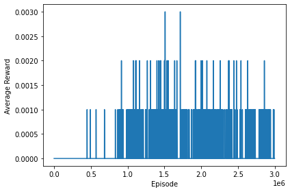
The clearest data is in the average returns. We can see that over the training steps it goes up, and it consistently stays up. We can see that the agent consistently reaches the goal state with an average reward of 0.10 per 1000 episodes after about half a million episodes.
Please note, the figure above represents the **intrinsic rewards **given by the environment. Shaped rewards were not used to generate this figure.
Comparison of custom Q-Learning algorithm with Deep Q-Learning
Our agent that was deployed using Deep Q-learning and standard q-learning environments never managed to reach the goal state. We can see that in Figure 1.2 (it shows a line chart with shaped rewards but the agent never managed to reach the goal state) and in Figure 1.5 the agent never gets a reward from the environment. Figure 1.6 shows that the reward consistently goes up and stays up after around half a million episodes. While the average reward ratio is not that great, we have to consider the complexity of the problem, i.e, in order to solve the board randomly we would need to take 9 steps right and 9 steps down at worst, which comes out to 1/(4¹⁸) or 1/68719476736. This is 4¹⁰ times or 10,48,576 times more unlikely. The is_slippery parameter makes the problem significantly harder for a 10* 10 board.
If we take into consideration the training time for both the q-learning algorithm and the neural network, the q-learning again comes out on top. It took Deep Q-Learning around 3 hours to run for 10000 games, while it took Q-Learning 8 minutes to run for 3 million episodes. We can say that the Q-Learning method is superior to the Neural Network method for reinforcement learning based on the time complexity and average rewards returned from the environment.
Conclusion
Using OpenAI gym, a FrozenLake v1 environment with a 10*10 board was successfully created. Deep Q-Learning was used to implement a neural network, which was then deployed for 10,000 episodes. While the agent was never able to obtain intrinsic rewards from the environment, we did observe reward progression for shaped rewards over time. Q-Learning was also used to power the game. To accurately assess the effectiveness of our custom algorithm in Q-Learning, we ran it in both scenarios, namely when the agent is aware of the reward location and when the agent is unaware of the reward location. We were able to see the agent consistently reaching the goal state after about half a million episodes of training using our enhancements to the standard Q-Learning method.
References
-
Github: https://github.com/nandangrover/reinforcement_frozenlake
-
Anderson, C. 1986, Learning and Problem-Solving with Multilayer Connectionist Systems (Adaptive, Strategy Learning, Neural Networks, Reinforcement Learning), PhD thesis, University of Massachusetts Amherst.
-
B. Jang, M. Kim, G. Harerimana and J. W. Kim, “Q-Learning Algorithms: A Comprehensive Classification and Applications,” in IEEE Access, vol. 7, pp. 133653–133667, 2019, doi: 10.1109/ACCESS.2019.2941229.
Related Posts
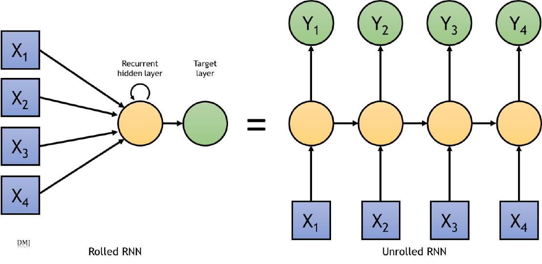
RNN for sequence-to-sequence classification
In order to understand a sequence of information we need to understand each input of data based on the understanding of previous data.
Read more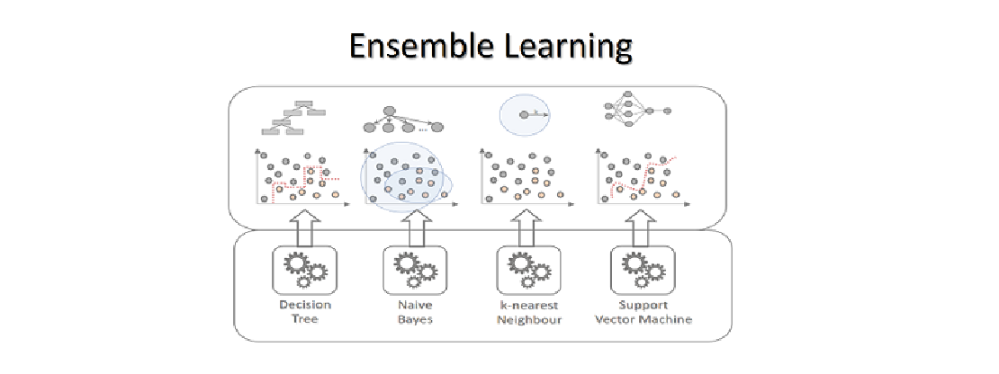
Learning based models for Classification
Thousands of learning algorithms have been developed in the field of machine learning. Scientists typically select from among these algorithms to solve specific problems.
Read more
Convolution Neural Nets and Multi-Class Image Classification
In 2015 the idea of creating a computer system that could recognise birds was considered so outrageously challenging that it was the basis of this XKCD joke .
Read more